Tutorials
Short, progressive, runnable tutorials for the euroflood library. They read the
published index (zero config: pip install "euroflood[viz]" and go) and follow one place
throughout: Zutphen, a Hanseatic town on the river IJssel in the Netherlands, whose
recurrent high-water flooding makes for a rich, interesting catalogue.
-
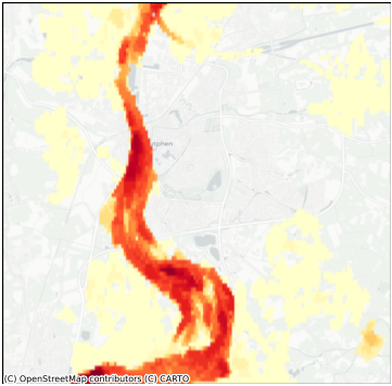
The whole idea in a few lines: query →
.plot(), straight from the index. -
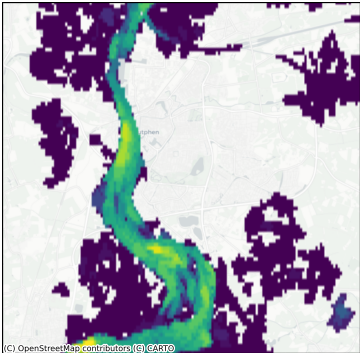
Query by place / bbox / point /
shape; filter by time; it's a GeoDataFrame. -
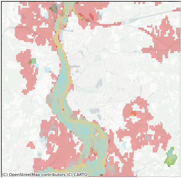
Recurrence heatmaps, per-event footprints, and interactive folium maps.
-
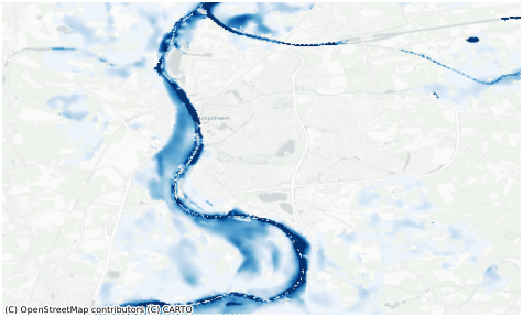
.download()→ depth rasters →DepthRaster/.stats()/.summary(). -
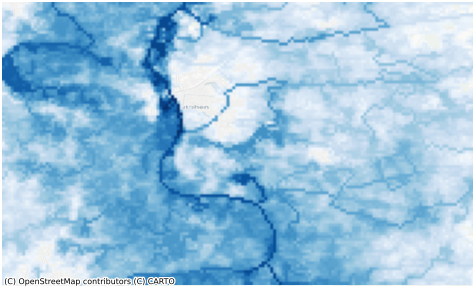
Modelled GLOFAS flood-hazard maps by return period (static + interactive).
-
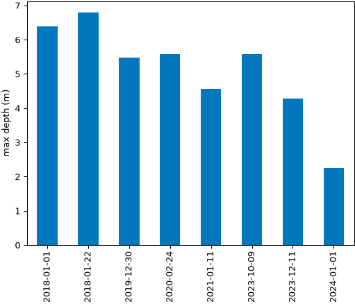
Rank events, estimate exposure, compare depths across events.
-
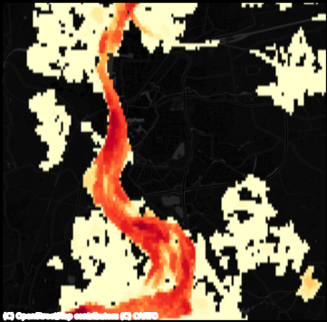
The
eurofloodcommand line, every setting, and offline / HPC use.
Run them yourself
pip install "euroflood[viz]"
jupyter lab examples/             # open the .ipynb, or:
python examples/01_quickstart.py  # the paired .py runs top-to-bottom as a script
Each tutorial is a jupytext pair: the .py is the
readable source of truth, paired to a .ipynb with rich outputs.