Concepts: how the index works

This page explains the one idea that makes the rest of EuroFlood click: how a huge, un-indexed archive of flood rasters becomes a query you can run in milliseconds and a few megabytes. You don't need this to use the library, but it explains why floods() is cheap, why recurrence and footprints need no download, and what all the files in the cache are.

The problem

The JRC / CEMS-EFAS archive is ~3,280 satellite flood-depth GeoTIFFs (~18.9 GB of depth rasters), distributed through a flat HTTP directory with no API, catalogue, or spatial index. The only geolocation you get without opening a file is a centroid encoded in its filename, and a single event file can contain flooded areas up to 2,870 km apart, so that centroid cannot represent the event. Filtering by filename therefore misses most events relevant to a place: a generous 2° buffer recovers at most ~48% of events, and precision falls to ~10% at city scale.

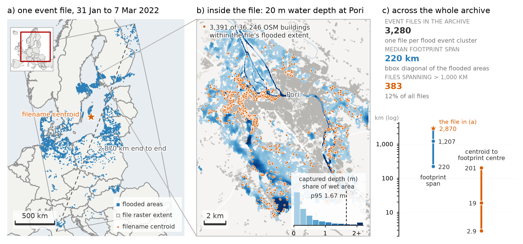
The archive is open in principle but hard to query in practice. EuroFlood precomputes an index so that "which floods hit Zutphen, and when?" becomes a single small raster read instead of a scan of every tile.

The building blocks

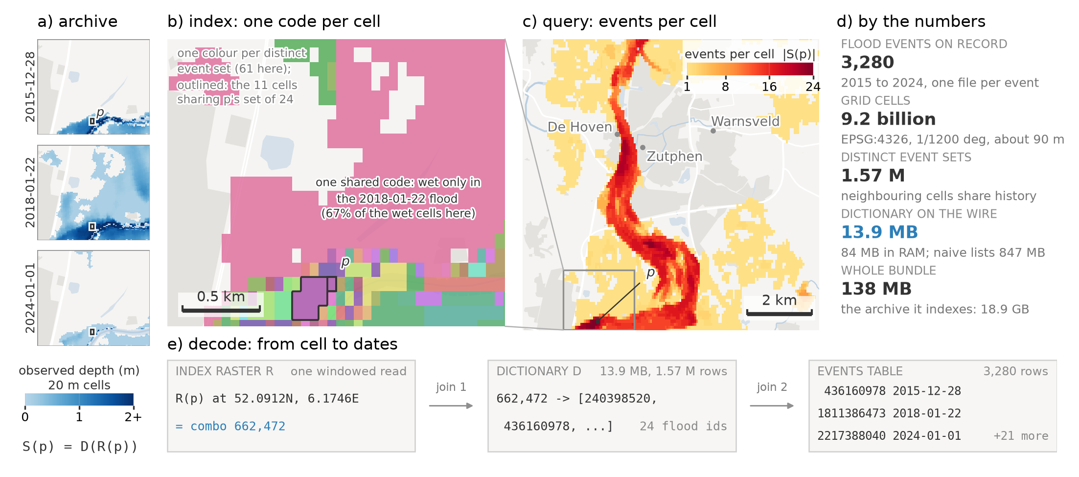
The whole index is three artifacts (a raster, a dictionary, and a table), built and decoded as shown below. The rest of this section walks through each piece.

1. A global grid

All maps are resampled onto one fixed lat/lon grid: EPSG:4326 at 1/1200° (≈3 arc-sec, ≈90 m pixels), covering Europe. (The source depth rasters are native 20 m; the index trades that resolution for a compact, uniform grid.) Every pixel has a stable (row, col) address, so "the same place" means "the same pixel" across all events.

2. The index COG: a pixel is a set of events

The index is a single Cloud-Optimized GeoTIFF (europe_flood_index.tif) on that grid. Each pixel holds a uint32 combo_id:

• 0: never flooded (the vast majority; the COG is sparse and compresses to 124 MB).
• N > 0: a combination id, a stable handle for the exact set of flood events that flooded this pixel.

Many pixels share the same set of events, so there are far fewer distinct combo_ids than pixels. That's what keeps the index small.

Why ~138 MB is enough

Europe is ~9.2 billion grid cells. Only 82.6 million (0.9%) were ever wet, and those resolve to just 1.57 million distinct event combinations. So instead of a dense 37 GB raster, or ~847 MB of explicit per-cell event lists, the index stores a 124 MB COG + a 13.9 MB dictionary + a 0.3 MB events table: about 138 MB in total, versus ~18.9 GB of source depth rasters.

3. The dictionary: combo_id → flood_ids

A small sorted GeoParquet (flood_dictionary.parquet) maps each combo_id to the list of flood-event ids that produced it:

combo_id  ->  flood_ids
   42     ->  [811, 1290]        # this combo = events 811 and 1290
   43     ->  [811]

4. The events table: flood_id → metadata

A tiny events.parquet maps each flood_id to its metadata (start/end date, year, cluster, source filename + download URL). Storing metadata once here, instead of repeating it inside every combo, keeps the dictionary + events table to ~14 MB with no information loss.

flowchart LR
    P["Index COG pixel<br/>combo_id = 42"] --> D["Dictionary<br/>42 → [811, 1290]"]
    D --> E1["events.parquet<br/>811 → 2015-11-30, WD_MERGE_…tif"]
    D --> E2["events.parquet<br/>1290 → 2019-09-12, WD_MERGE_…tif"]

Discover → Extract

EuroFlood follows a two-stage model. Discovery finds which events affected a region, when they occurred, and how often cells were inundated, using only the ~138 MB index. Extraction then retrieves native-resolution depth rasters, but only for the events you selected. So a query resolves in two cheap steps, then an optional extract:

1. Resolve the region: a place name (geocoded), bbox, point+radius, or shapefile becomes an ROI polygon. shape="bbox"/"hull" optionally regularizes it to a bounding rectangle / convex hull (handy when an admin boundary follows a river), and buffer_m grows it.
2. Discover: mask the index COG to the ROI (reading only that window), collect the distinct combo_ids, expand them to flood_ids via the dictionary, and join the events table for metadata. The result is a FloodFrame, one row per event. No depth rasters are touched.
3. Extract (opt-in): .download() fetches and crops only the source depth GeoTIFFs for the events you selected.

That's why floods("Zutphen, Netherlands") transfers a few MB and returns instantly, while the actual depth data is fetched only when you ask.

Local vs. remote index

The same index can live locally or be streamed:

• Remote (default for the published index): the COG is read a window at a time over HTTP via GDAL's /vsicurl, and only the ~14 MB dictionary + events tables are cached on first use (SHA-256-verified). A query downloads a few MB, never the whole index. Controlled by EUROFLOOD_INDEX_MODE / EUROFLOOD_INDEX_BASE_URL.
• Local: everything is read from the cache directory. euroflood mirror index pulls the full ~138 MB bundle once for fully-offline / HPC use.

Hazard has a parallel switch, hazard_mode (auto/local/remote), and both collections share a master EUROFLOOD_OFFLINE=1 / euroflood.offline() toggle that forces everything cache-only and the geocoder offline. Stage data with euroflood mirror index|floods|hazard|all and gate readiness with euroflood verify … --deep. In local/offline mode a missing tile raises a clear error naming the mirror command to run, never a silent partial result.

What the visualizations reuse

Because the index already encodes which events hit each pixel, several views come for free, no download:

• Recurrence heatmap: per pixel, len(flood_ids) is exactly how many times it flooded. Darker = more floods.
• Per-event footprints: an event's extent is the union of pixels whose combo_id includes that event; .footprints() returns one geometry per event.
• Depth map: the only view that needs the actual raster, hence depth=True downloads it.

So most views cost nothing beyond the query; only the depth map touches the network:

Call	Network / disk	Shows
cat.plot() / .explore()	none	recurrence heatmap (historic) / context (hazard)
cat.plot(event_id=…)	none	one event's footprint
cat.footprints() / cat.plot(footprints=True)	none	each event's extent (data + map)
cat.plot(depth=True, …)	downloads rasters	actual water-depth map
ef.plot_depth(path)	none	a depth map from a downloaded GeoTIFF

See Tutorial 3: Visualize for the full gallery.

How complete, and how trustworthy

The index reconstructs the archive's event footprints exactly at its ~90 m grid: across 100 events sampled over all ten years, footprints decoded from the published index match an independent re-ingest of the source rasters with an IoU of 1.000: no missing or spurious cells, no missing or spurious events. Queries also return byte-identical results whether streamed from the public host, a local mirror, or a private replica.

And the index is fast because discovery reads only a window of it. Computing recurrence for the whole Netherlands, for example, is a 15.2 MB windowed read of the index versus 3.9 GB of source rasters, a 254× reduction; marginal queries transfer just 0.12–0.91 MB.

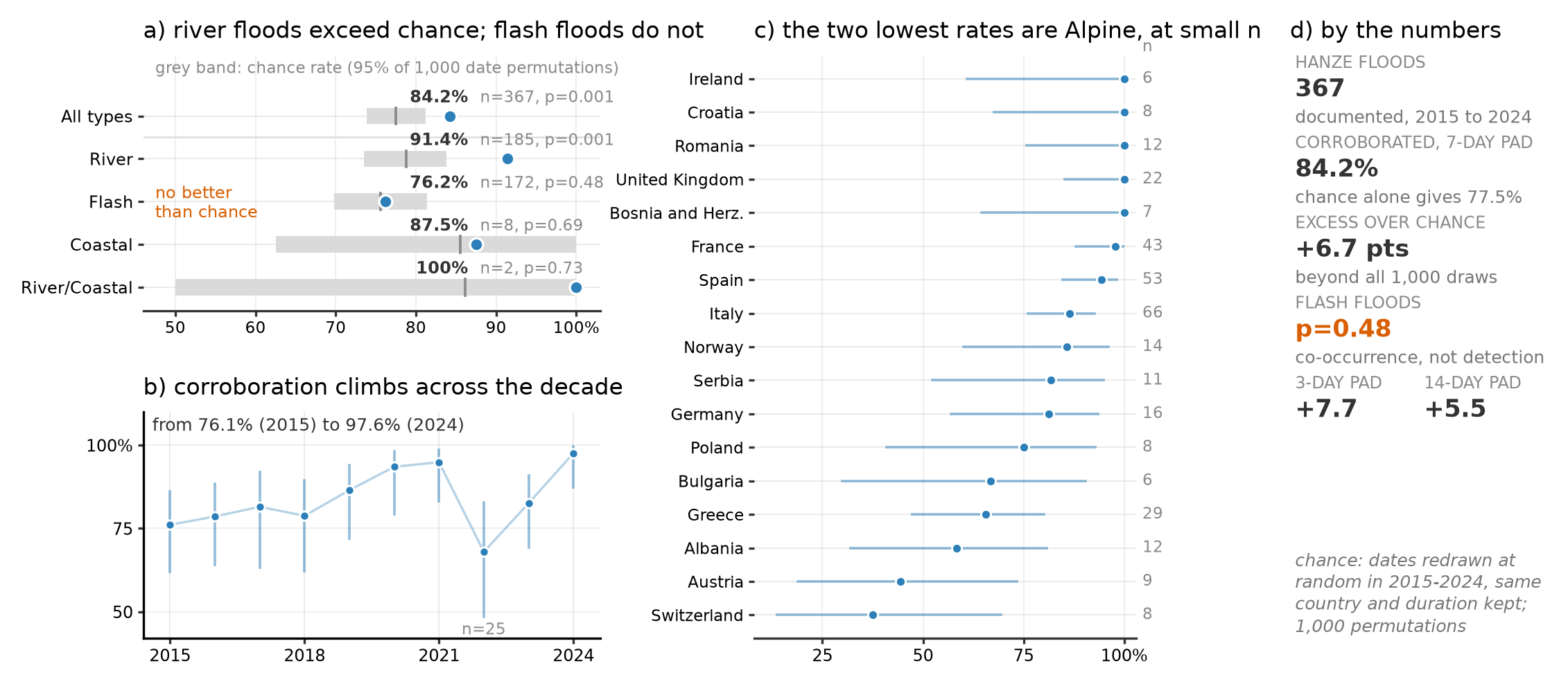
How complete is the archive itself? Compared against HANZE, an independent European flood-impact database (367 floods, 2015–2024), 84.2% of documented floods coincide with an archived event in the same country within a week, well above the ~77.5% expected by chance. The signal is strongest for river floods (91.4%) and indistinguishable from chance for flash floods (76.2%), and completeness rises over the decade (76.1% in 2015 → 97.6% in 2024).

Interpreting your results

The index answers "where and when has flooding been detected?", not "where has flooding occurred?" A few things to keep in mind:

Detected ≠ complete

An absent or spatially limited footprint does not mean flooding was absent. Sentinel-1 under-detects short-lived, urban, vegetated, and topographically confined events (see the Valencia DANA and Baltic surge case studies).

Recurrence is a detection count, not a return period

A recurrence value is how many archived events touched a cell, not a hydrological frequency or return period. Two nearby cells can differ simply because of when satellites happened to observe them.

Use the index for discovery, the 20 m rasters for measurement

The any-wet resampling that keeps the index lossless also enlarges footprints: a median 1.49× area inflation (mean 1.53; 10th–90th percentile 1.27–1.82) relative to the native 20 m wet area. Use the index for discovery, recurrence, and spatial selection; compute inundated area, depth, and volume from the downloaded 20 m rasters (.download().stats()).

Modelled GLOFAS hazard maps and observed footprints are different representations (a return-period scenario versus what a satellite saw on specific dates), so treat them as complementary, not as validations of each other. Depths themselves are reconstructed (FLEXTH), accurate to roughly a decimetre (RMSE 0.28–0.62 m).

The cache, at a glance

A built/mirrored index bundle contains:

File	What it is
europe_flood_index.tif	the sparse COG (pixel = combo_id)
flood_dictionary.parquet	combo_id → flood_ids
events.parquet	flood_id → metadata
dictionary_meta.json	schema/version/layout
manifest.json	provenance + checksums (the publish/validate contract)

Producers build these with mirror → ingest → build-index; see the HPC Runbook.